Rapp. Comm. int. Mer Médit., 37,2004
127
CORRECTION OF MODELED SEA SURFACE WIND IN ORDER TO IMPROVE WAVE FORECAST
A. Murashkovsky*, I. Gertman
Israel Oceanographical and Limnologial Research, National Institute of Oceanography, Haifa 31080, Israel - * amur@ocean,org.il
Abstract
A method for correcting wind input to WAM model is proposed in order to re?ect wind gusts, otherwise not present in the atmospheric
models output. The method is based on wind field vorticity analysis and does not require any external data. The wave forecast resulting
from winds corrected by this method was compared to real data, as well as to forecasts resulting from a different correction technique.
Keywords: wind gusts, WAM model
Introduction
Operational wave forecasting system based on WAM model for the
Eastern Mediterranean was implemented in IOLR since fall 1997 [1].
The results of the wave forecast and hindcast produced by the system
were compared to true data from Hadera GLOSS station from the
beginning of the project.
From the very beginning the comparisons showed that H
s
is
underestimated and this fault increased with H
s
increases. The
problem of the wave model underestimating H
s
isn’t new, it was
addressed before, e.g. Cavalieri [2], and it is attributed to negative
errors in closed basins. However, it was suggested that during severe
storms another factor may in?uence the H
s
growth, namely wind
gusts, which, typically, are not represented in the output of
meteorological models.
Several methods have been suggested for the introduction of wind
gustiness into wave model input. Abdalla and Cavalieri [3] used
fluctuations represented by Gaussian process, characterized by
coherence in time. Another method proposed adding a constant factor
to the wind field. Wave Watch III, as of ver. 1.18 [4] used term
dependent on T
air
-T
w
difference to represent atmospheric instability
and calculate an effective wind speed.
This paper proposes a new method, based on the assumption that
most severe wind gusts occur during the passage of atmospheric
fronts, and are indicated by significant changes in the wind direction.
Methods and materials
Hess [5] defines an atmospheric front as zone of rapid transition
from one temperature to another. It also noted that significant wind
direction changes occur in frontal zones. The frontal zones are
characterized by strong atmospheric instabilities, often resulting in
severe weather, and are usually accompanied by strong wind gusts.
The quantitative characteristic of vector field direction change is its
curl, which leaded to defining “gustiness” of the wind field as
The actual correction was calculated using measured data at Hadera
GLOSS station, and resulted in
Results and discussion
Two sources of wind input were used during the verification of the
method: the SKIRON forecasting system from University of Athens
(output every 6 hours, 0.2x0.2ş resolution); and the Bracknell model
by UKMO (output every 6 hours, 0.833x0.566ş resolution). Both T
air
-
T
w
and wind vorticity correction techniques were applied and the
results were compared to the measured data. The immediate result of
the comparisons revealed that the impact of both methods on low
resolution wind was insignificant, so that only SKIRON wind was
utilized subsequently.
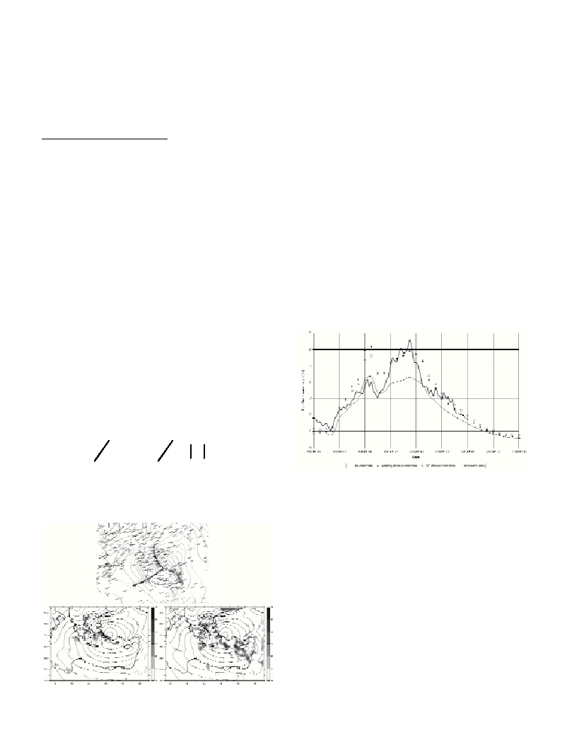
On the synoptic map three frontal zones are clearly visible: a hot
one and two cold ones. Predictably dT derived correction is very small
in the hot frontal zone, while the vorticity derived correction produces
significant values. The correction based on vorticity also increased
near the shores, where wind changes its direction.
Another comparison was carried out by using the WAM model for
the Levantine basin to produce wave hindcast with wind input
corrected by various methods. The results were compared to data
measured at Hadera GLOSS station. It is clear that both methods
improve the forecasts significantly, when compared to forecasts
produced with uncorrected wind input. The preliminary studies
confirm that both methods produce similar results, while vorticity
derived technique requires less data.
Fig. 2. Comparison of significant wave height with wind input produced
by different methods.
Acknowledgments
We want to thank sincerely to Prof. G. Kallos from SKIRON group
for providing us with wind data for this work.
References
1-Gertman I. Rosen D.S., Sandler K. and Raskin L., 2000. Comparison
of two years of wind and wave hindcast via WAM based operational
forecasting system versus field and other models data. Proceedings of 6th
international workshop on wave hindcast and forecast. pp 91-98.
2-Cavalieri L., 1994. Orographic Effects, pp. 293-294. In:Komen G.J
(ed) Dynamics and Modeling of Ocean Waves. Cambrige Univ. Press,
New York.
3-Abdalla S. and Cavalieri L., 2002. Effect of wind variability and
variable air density on wave modeling. Journal of geophysical research,
107: 17-1 – 17-17.
4-Tolman H. L. 1999a. User Manual and system documentation of
Wavewatch-III, ver 1.18. OMB Contribution No 166.
5-Hess S. L., 1959. Introduction to theoretical meteorology. Holt,
Rinehart and Winston, New York.
65
.
0
)
(
*
399
.
0
+
=
G
Ln
G
corr
10
10
10
)
(
)
(
U
U
U
U
U
G
Y
X
r
r
r
r
r
·
?
?
?
?
?
?
?
×
?
?
+
?
×
?
?
=
Fig. 1. Frontal zone wind correction, calculated by different methods
during severe storm. Top : synoptic map; bottom left : dT derived
correction; bottom right : vorcity derived correction.