Rapp. Comm. int. Mer Médit., 37,2004
144
ANNUAL TO DECADAL SEA LEVEL VARIATION (35N-52N, 10W-13E)
E. Tel* and M. J. García
Instituto Espańol de Oceanografía (IEO), Madrid, Spain - *Elena.tel@md.ieo.es, Mjesus.garcia@md.ieo.es
Abstract
Monthly mean sea level values from tide gauges have been analysed for the area (35N-52N, 10W-13E) in the ESEAS-RI (WP3.1) project
framework. Standard quality control procedures have been applied to the data and Fourier and Empirical Ortogonal Functions (EOF)
analysis has been performed to the data set. Stations have been grouped in 6 region (number of significant series has been reduced from
35 to 10) obtained by EOF.
Keywords: EOF, time series analysis, mean sea level.
Monthly mean sea level values from the tide-gauge stations located
in the area (35N-52N, 10W-13E) are analysed. Data come from the
Permanent Mean Sea Level Service (PSMSL). Series of Ceuta,
Cadiz, Algeciras, Tarifa and Malaga come from the IEO Data Centre
because during the last years a big effort in quality control has been
done, in particular in homogeneization of time series. In some cases,
series has been cut in shorter ones because there are shifts along
them.
Linear trend are calculated and removed at each station. Some trend
values are very suspicious, probably because the sea level signal is
contaminated by the instability of tide-gauges location. The clearest
example is Dieppe, where its trend is bigger than other records in its
area. Negative trend at P.St. Gildas and Gibraltar correspond to
?agged records with stability problems. In addition, trend values
depend strongly on length records. The GIA rate (1) has been used to
remove the Post Glacial rebound. Annual cycles have been calculated
too, and removed by subtracting means monthly values to the record
anomaly.
Fourier analysis has been performed in order to identify long-
period significant cycles in the detrended and deseasonalizated series.
The contribution of a given frequency to the total variance of the time
series is a measure of the importance of that particular frequency
component in the observed signal.
EOF analysishas been done to classify the set of variables in
several groups that keep common characteristics and behaviour. These
groups are defined performing an EOF of a bigger area and selecting
the more explicative variables. St.Helier, P.St.Gildas and Cadiz
stations are eliminated in this analysis due to stability problems. In
each group, the first EOF accounts for the main part of total variance
in the data, the second EOF holds the maximum variance that has not
been accounted by the first EOF, and so on. The kept EOF factors at
this work explain, at least, 75% of total variance. As a result of this
analysis, an important data reduction has been achieved. This few new
variables can be used for interpretational purposes or in further
analysis.
Table 1. Groups and EOFs found in the performed analysis.
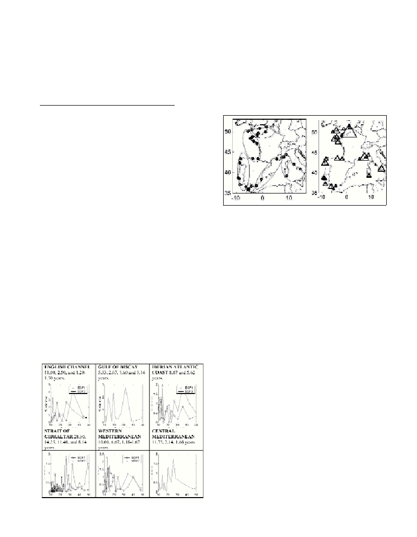
Fig. 1. Regions defined by EOF and trend values with the corresponding
PGR corrections.
References
1-Peltier, W.R., ICE4G (VM2), 2001. Glacial Isostatic Adjustment
Corrections. In : Douglas, B.C., Kearney, M.S., and S.P. Leatherman
(eds.), Sea Level Rise; History and Consequences. Academic Press.